QIP random circuits mystery resolved! Part 1

Thank you QIP audience! On Tuesday, I gave a presentation on this paper
Phys. Rev. A 95, 042306 (2017)
https://arxiv.org/abs/1612.02689
I had some great questions, but in retrospect don’t think my answers were the best. Many questions focused on how to interpret results showing that random circuits improve on purely unitary circuits. I often get this question and so tried to pre-empt it in the middle of my talk, but clearly failed to convey my point. I am still getting this question every coffee break, so let me try again. Another interesting point is how the efficiency of an optimal compiler scales with the number of qubits (see Part 2). In what follows I have to credit Andrew Doherty, Robin Blume-Kohout, Scott Aaronson and Adam Bouland, for their insights and questions. Thanks!

First, let’s recap. The setting is that we have some gate set $\mathcal{G}$ where each gate in the set has a cost. If the gate set is universal then for any target unitary $V$ and any $\epsilon > 0$ we can find some circuit $U = G_1 G_2 \ldots G_n$ built from gates in $\mathcal{G}$ such that the distance between the unitaries is less than $\epsilon$ . For the distance measure we take the diamond norm distance because it has nice composition properties. Typically, compilers come with a promise that the cost of circuit is upperbounded by some function $f(\epsilon) = A \log ( 1 / \epsilon)^\gamma$ for some constants $A$ and $\gamma$ depending on the details (see Part 2 for details).

The main result I presented was that we can find a probability distribution of circuits $\{ U_k , p_k \}$ such that the channel

$\mathcal{E}(\rho) = \sum_k p_k U_k \rho U_k^\dagger$

is $O(\epsilon^2)$ close to the target unitary $V$ even though the individual circuits have cost upper bounded by $f(\epsilon)$ . So using random circuits gets you free quadratic error suppression!

But what the heck is going on here!? Surely, each individual run of the compiler gives a particular circuit $U_k$ and the experimentalist know that this unitary has been performed. But this particular instance has an error no more than $\epsilon$ , rather than $O( \epsilon^2)$ . Is it that each circuit is upper bounded by $\epsilon$ noise, but that somehow the typical or average circuit has cost $O(\epsilon^2)$ . No! Because the theorem holds even when every unitary has exactly $\epsilon$ error. However, typicality does resolve the mystery but only when we think about the quantum computation as a whole.

Each time we use a random compiler we get some circuit $U_k = V e^{i \delta_k}$ where $e^{i \delta_k}$ is a coherent noise term with small $|| \delta_k || \leq O(\epsilon)$ . However, these are just subcircuits of a larger computation. Therefore, we really want to implement some large computation

$V^{(n)} \ldots V^{(2)} V^{(1)}$ .

For each subcircuit compiling is reasonable (e.g. it acts nontrivially on only a few qubits) but the whole computation acts on too many qubits to optimally compile or even compute the matrix representation. Then using random compiling we implement some sequence

$U^{(n)}_{a_n} \ldots U^{(2)}_{a_2} U^{(1)}_{a_1}$

with some probability

$p_{a_n}^{(n)} \ldots p^{(2)}_{a_2} p^{(1)}_{a_1}$ .

OK, now let’s see what happens with the coherent noise terms. For the $k^{th}$ subcircuit we have
$U^{(k)}_{a_k} = V^{(k)} e^{i \delta_{a_k}^{(k)}}$

so the whole computation we implement is

$U^{(n)}_{a_n} \ldots U^{(2)}_{a_2} U^{(1)}_{a_1} = V^{(n)} e^{i \delta_{a_1}^{(n)}}\ldots V^{(2)} e^{i \delta_{a_2}^{(2)}} V^{(1)} e^{i \delta_{a_n}^{(n)}}$

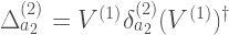
We can conjugate the noise terms through the circuits. For instance,

$e^{i \delta_{a_2}^{(2)} } V^{(1)} = V^{(1)} e^{i \Delta_{a_2}^{(2)}}$

where

$\Delta_{a_2}^{(2)}= V^{(1)} \delta_{a_2}^{(2)} (V^{(1)})^\dagger$ .

Since norms are unitarily invariant we still have

$||\Delta_{a_2}^{(2)}|| = || \delta_{a_2}^{(2)} || \leq O(\epsilon)$

Repeating this conjugation process we can collect all the coherent noise terms together

$U^{(n)}_{a_n} \ldots U^{(2)}_{a_2} U^{(1)}_{a_1} = (V^{(n)} \ldots V^{(2)} V^{(1)} ) ( e^{\Delta_{a_n}^{(n)}} \ldots e^{\Delta_{a_2}^{(2)}} e^{\Delta_{a_1}^{(1)}})$

Using that the noise terms are small, we can use

$e^{\Delta_{a_n}^{(n)}} \ldots e^{\Delta_{a_2}^{(2)}} e^{\Delta_{a_1}^{(1)}} \sim e^{\Delta}$

where

$\Delta = \sum_k \Delta_{a_k}^{(k)}$

Using the triangle inequality one has

$|| \Delta || \leq \sum_k || \Delta_{a_k}^{(k)}|| \leq n O(\epsilon)$ .

But this noise term could be much much smaller than this bound implies. Indeed, one would only get close to equality when the noise terms coherently add up. In some sense, our circuits must conspire to align their coherent noise terms to all point in the same direction. Conversely, one might find that the coherent noise terms cancel out, and one could possibly even have that $\Delta = 0$ . This would be the ideal situation. But we are talking about large unitary. Too large to compute otherwise we would have simulated the whole quantum computation. For a fixed $\Delta$ , we can’t say much more. But if we remember $\Delta$ comes from a random ensemble, we can make probabilistic arguments about its size. A key point in the paper is that we choose the probabilities such that the expectation of each random term is zero:

$\mathbb{E} ( \Delta_{a_k}^{(k)} )= \sum_{a_k} p^{(k)}_{a_k} \Delta_{a_k}^{(k)} = 0$ .

Furthermore, we are summing a series of such terms (sampled independently). A sum of independent random variables are going to convergence (via a central limit theorem) to some Gaussian distribution that is centred around the mean (which is zero). Of course, there will be some variance about the mean, but this will be $\sqrt{n} \epsilon$ rather than the $n \epsilon$ bound above that limits the tails of the distribution. But this gives us a rough intuition that $\Delta$ will (with high probability) have quadratically smaller size. Indeed, this is how Hastings frames the problem in his related paper arxiv1612.01011. Based on this intuition one could imagine trying to upper bound $\mathbb{E} ( || \Delta|| )$ and make the above discussion rigorous. Indeed, this might be an interesting exercise to work through. However, both Hastings and I instead tackled the problem by showing bounds on the diamond distance of the channel, which implicitly entails that the coherent errors are composing (with high probability) in an incoherent way!