I not posting here as much as I used to. But I am more active on the Riverlane website. Some of my post on the Riverlane site include:
https://www.riverlane.com/news/introducing-the-world-s-first-low-latency-qec-experiment
https://www.riverlane.com/blog/2024-s-qec-highlights-aka-the-12-days-of-qechristmas
https://www.riverlane.com/blog/how-to-develop-the-quantum-error-correction-stack-for-every-qubit
Category: Uncategorized
Quantifying quantum speedups
I just finished a fun collaboration arXiv2002.06181 on magic monotones, classical simulation and related results. The paper is pretty long (23+4) and we had to write a 3-page summary in order to submit to TQC conference. So if you want to get an overview or find out why you should read the full paper, our TQC abstract is a good starting place.
The quantum ENIAC and Schrodinger’s glass
Language is wonderfully subtle. Two sentences can mean the same thing but leave the reader with completely different impressions. Everyone can appreciate that “The glass is half empty” and “The glass is half full” actually mean the same thing. Yet, they leave different impressions on the reader.

Sabine Hossenfelder’s recent Guardian column on quantum computation is titled
Quantum supremacy is coming. It won’t change the world
and it muses on the impending announcement of quantum supremacy. Soon, someone (possibly Google) is going to announce that they have used a quantum computer to perform a particular calculation faster than our fastest conventional supercomputers! Sabine’s spin is that Schrodinger’s glass is very much, half-empty. Even worse it is half empty with gone off milk.
Should you believe her?
We are in the midst of a surge of optimism, investment and frequent hype around quantum computation. Sabine’s column is a refreshing change to the worst of the hyperbole currently circulating. It has a similar, acerbic tone that she also takes in her critique of particle physics. It is fun to read and I’ve enjoyed many of her blog articles on the disconnect between experiment and theory in the high energy physics community. Of course, a balanced perspective sits somewhere between the extremes of Sabine’s pessimism and those overpromising on quantum computation.
Let’s start with the headline. If we tweak it slightly to
Quantum supremacy is coming. It won’t change the world tomorrow
then she is absolutely right. The day after you won’t notice any difference.
But she insinuates that quantum computers will never change the world, which is unwarranted and absurd given the parallels she draws with early conventional computers. She compares the coming generation of quantum computers with an early computer ENIAC that was publically announced in 1946. It did take about 35 years from ENIAC until people could have their own personal computer (PC) at home, and 60 years until most people started carrying smart phones in their pockets! This is arguably the most rapid and significant change in human history, so the comparison is a bit bizarre.
It is difficult to see why Sabine makes the comparison with ENIAC, maybe the point is that many people are promising useful quantum computers in less than 35 years. But long before you got your first PC or smartphone, computers were having a huge (though often invisible) effect on our lives. Sabine suggests that ENIAC itself had no impact itself. However, before the public announcement of ENIAC’s existence, it was used to target artillery and also to design the first atomic bomb. Around this time, simple computing devices also played a crucial role in the growing telephone network. If 2019 was the year of the quantum-ENIAC and history repeats itself, then this would be a monumental event. As many others have pointed on the comments section of her article, the analogy with ENIAC is both flawed and fails to support her main headline.
Let’s set aside historical analogies. What else does Sabine say:
Quantum supremacy will be a remarkable achievement for science. But it won’t change the world any time soon. The fact is that algorithms that can run on today’s quantum computers aren’t much use. One of the main algorithms, for example, makes the quantum computer churn out random numbers. That’s great for demonstrating quantum supremacy, but for anything else? Forget it.
Here Sabine is referring to a specific task that many companies are planning to use as their first test of how the quantum computer performs against a conventional computer. She makes a strong point here. The so-called cross-entropy benchmarking tests are just as dull and technical as the name sounds.
To me, this is a benchmarking test. When a quantum device passes the test, it tells you that technology has reached a new level of maturity. Sabine is also right that cross-entropy benchmarking does not have any practical applications and no-one would pay a billion pounds for a device that could only perform this task. However,…
What the cross-entropy benchmarking test really shows is that the technology is sufficiently mature that it is worth running other programmes on the hardware. Much more exciting is to use a quantum computer solve problems in chemistry and material science. Computing power is a definite bottle-neck point in the design of drugs and materials, so we’d like to try and solve these problems on a quantum computer. In the near future (soon after passing the cross-entropy benchmarking tests) we can start our first attempts using a heuristic algorithm called VQE (the variational quantum eigensolver). Possibly, the 50-100 qubit devices coming soon would provide commercially useful solutions in this sector.
Why am I hedging with words like “possibly” and what does “heuristic algorithm” mean. I want to give a balanced perspective, so let explain what I mean here. First, let’s check the Wikipedia page for heuristic
The objective of a heuristic is to produce a solution in a reasonable time frame that is good enough for solving the problem at hand. This solution may not be the best of all the solutions to this problem, or it may simply approximate the exact solution. But it is still valuable because finding it does not require a prohibitively long time.
This doesn’t sound too bad. Indeed, the vast majority of conventional computing software is built on a mountain of heuristics so they are pretty useful. However, often it is hard to predict the performance of a heuristic until you’ve run it on an actual device. However, we can design heuristics and test them for 20-30 qubit on our laptop using an emulation of a quantum computer. So for these small sizes, your laptop could predict exactly what the quantum computer would do when you run the heuristic. This gives you a decent idea what will happen when you run the heuristic on a 50 qubit quantum computer.
This is a design process happening now, for instance by the company RIVERLANE that I work for part-time. But there is some uncertainty in the extrapolation from 20-30 qubits to 50-100. This all tells us that there is a chance to solve some exciting chemistry problems in the near-term, but the technology might need to be more mature before we see any big payoffs.
Why use heuristics? In the near future, quantum computers won’t be perfect and as Sabine notes “The trouble is that quantum systems are exceptionally fragile”. The longer the computation, the more the noise accumulates. Consequently, we are currently limited to short, heuristic computations.
There are many quantum algorithms where we can give a mathematical proof of how the quantum computer will perform! This sounds better than using a heuristic. But these algorithms are much bigger computations than the heuristics that I mentioned above. In these larger-scale algorithms, the noise accumulation problem can be avoided by continually correcting errors. Though this quantum error correction procedure does use up some of our qubits, further adding to the required scale of the device.
Okay, so how many good quality qubits would I need so that I can say with 100% certainty that the quantum computer would change the world. Here Sabine says:
To compute something useful – say, the chemical properties of a novel substance – would take a few million qubits. But it’s not easy to scale up from 50 qubits to several million.
A few million qubit is indeed what is estimated in some of the recent literature (see for example). There are two issues with this quote. First, it ignores the heuristic methods I mentioned earlier. Second, it suggests that it would be impossible to solve this problem with fewer than a million qubits! The number of qubits needed will depend on the quality of the hardware and the design of the algorithms and error correction methods. Come up with better designs of hardware or software and the numbers go down and the technology progresses. Only a few years ago, to solve the same chemistry problem our best estimates would have been closer to a billion qubits!
In the one million qubit blueprint, many of the qubits are busy removing noise. This would allow the quantum computer to run long enough to compute reliably. Sabine does not seem aware of this point as she says that
Even when housed in far-flung shelters and accessed through the cloud, it is not clear that a million qubit machine would ever remain stable for long enough to function.
She is missing the point that a million qubits are budgeted for precisely to provide a guarantee that it will remain stable for long enough. On the other hand, for the smaller 50-100 qubit computer, the stability issue is more nuanced because everything is heuristic and without error correction.
The technological and algorithmic obstacles are tough and challenging. But as we work hard on these problems, we see two things happen: hardware developers release better devices with more qubits and less noise; theorists come up with better designs that need fewer qubits. This is happening now, we are not stuck on any insurmountable problems.
Towards the conclusion of Sabine’s column she ponders
Researchers need to move on. They must take a good, hard look at the quantum computers they are building and ask how will they make them useful.
Again, Sabine states something factually correct but in a glass-half-empty tone. However, I am happy to report that this is exactly what we are doing. I have just got home from QEC2019, a 1-week conference in London (more info here) where we focused on how to make the quantum error correction components more efficient. The conference had theorists reporting new techniques and ideas for how to perform error correction. It also had experimentalists describing the latest hardware progress. Most people at QEC are pretty realistic and can see that the glass definitely contains 50% water / 50% air and the tap is still running.
Quantum dynamics goes Monte Carlo!
This post is a light summary of a project just published in Physical Review Letters. I am very pleased that this work got selected as an editor’s suggestion and that the legendary Dominic Berry was commissioned to write a Physics view-point. His viewpoint really is a superb summary and you should go read it now, then come back here!
on how best to simulate time evolution using a quantum computer, which can also be helpful with other tasks like finding the ground state energy of a Hamiltonian. The standard method is to Trotterize the dynamics, and in some situations this works quite well, but it struggles with Hamiltonians containing a large number of terms.
If a Hamiltonian has L terms then even the best known Trotter methods have a gate count scaling quadratically with L. This is especially problematic in molecular systems because an N electron/qubit system will have about N^4 terms in the Hamiltonians, so L^8 gates in the Trotterized approach. Since systems beyond the reach of classical computers have N>40, the numbers quickly become horrifying.
My new work proposes a protocol with no explicit L dependence in the gate count, so it performs much better for Hamiltonians with many, many terms. The key idea is to use randomness.
Before getting to the new ideas, let’s recap Trotterization using some simple pictures. In Trotterization, we divide the evolution into r Trotter steps. In the simplest version of Trotter, each step contains one gate for each term in the Hamiltonian as follows.
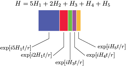
Each gate is a coloured block with the width indicating the duration of the pulse. The width of the blocks are proportional to the corresponding coefficients in the Hamiltonian. In the standard cost model, each of these blocks has unit cost, independent of the duration of the gate, so the above sequence has cost 5. Next, we repeat this r times to obtain a sequence illustrated by:
![]()
where here we have taken 10 Trotter steps. There are 5 gates per step and so 50 gates in the whole sequence. The black ticks are just to guide the eyes to the divisions between each step.
How to do better? The main idea is to use random compiling. Both me and Matt Hasting showed a couple of years ago that randomisation can be very useful in compiling quantum circuits. If your interested in this more general problem, I gave a talk at QIP at Delft. Childs, Ostrander, and Su have a paper where they suggest randomly permuting gates within each Trotter step, so for a particular sample you might get a sequence like
![]()
This does lead to improved performance but does not escape the L^2 dependence of the gate count, so still isn’t especially suited to Hamiltonians with very many terms.
In my paper, I proposed that we instead choose all the gates in the sequence independently (i.i.d) at random, with each block having the same width/duration. So every gate is of the form

where the width 
![]()
The colour refers to which 

There are two effects at work here. First, we see that in the original Trotter there were a lot of weak gates (yellow, green and purple) that were repeated in every step. One of the main savings is that these are consolidated. Second, the sequence is random and so any coherent noise effects are washed out into less harmful stochastic noise. This is a very subtle point that I’ve blogged on previously, so I won’t labour the point again other than to stress that the protocol only works if a different random sequence is used for every run of the quantum computer.
Remarkably, one finds the number of gates required is independent of the number of terms in the Hamiltonian! This is proved by Taylor expanding and careful bounding of errors, much like the proofs for standard Trotter. One difference is that instead of Taylor expanding a unitary we perform a Taylor expansion of an exponentiated Lindblad operator.
For technical details, you should see the paper. To wrap up here, I just want to add that the above random protocol (which I call qDRIFT) is very simple and there is plently of scope for more sophisticated ideas exploiting the same effects. Right away one can see that there is some waste in the above gate sequence; whenever you see subsequent gates of the same colour, they can be merged into a single gate. Applying such a merge strategy to the above, one would have the sequence:
![]()
which has only 16 gates!
Are quantum computers more powerful than classical computers and the stabiliser rank story. (part 1)
Of course, quantum computers are more powerful than classical computers, but how do you prove it! Until recently there was not much known except for some oracle separation results. In 2017, we got the already infamous Bravyi-Gosset-Koenig result that proved quantum computers can solve some problems in constant time that for a classical computer require logarithmic time. But we really want to know that quantum computers offer an exponential speedup such as Shor’s algorithm suggests.
Asking for a proof of an exponential speedup is a lot to ask for! We would need to show that all possible classical algorithms are incapable of efficiently simulating a quantum computer. This is really hard. But if we have a concrete family of classical algorithms, then surely we should try to understand if they could possibly offer an efficient simulation!
This brings us to stabiliser rank and related simulation methods. Let’s define some terms. Given a state 

Definition of stabiliser rank:
Suppose is a pure
  -qubit state. The exact stabilizer rank
  is the smallest integer
  such that can be written as
Suppose
is a pure -qubit state. The exact stabilizer rank is the smallest integer such that can be written as

for some 

These decompositions were first studied by Garcia- Markov-Cross and applications to simulation were first explored in more depth by Bravyi-Smith-Smolin. The Gottesman-Knill theorem allows us to efficiently simulate a Clifford circuit acting on a stabiliser state. This can be extended to simulation of an arbitrary state 


So if quantum computers are more powerful than classical computers, then we expect 
Surely, this is a simple statement that the quantum community should be able to prove. Surely, stabiliser rank simulators are not going to show BQP=BPP. Surely, surely we can prove the following conjecture:
The stabiliser rank conjecture:
For every nonstabiliser state, there exists a  such that
For every nonstabiliser state
, there exists a such that
holds for all integer
Clearly, one has that 

But when we consider 2 copies of the state we have

where

This is a decomposition with 3 stabiliser terms and so

for all single qubit


(see Sec V.A of arXiv_V1). The stabiliser rank grows linearly! Not exponentially, but linearly! OK, this scaling holds up until only five copies, but I find this remarkable. Incidentally, the proof has a nice connection to the fact that the Clifford group forms a 3-design. Beyond five copies, the numerics look exponential, but the numerics are heuristic, inconclusive and only go slightly further than five copies!
Do we have any lower bounds on stabiliser rank! Deep in Bravyi-Smith-Smolin (Appendix C) is tucked away a neat result showing that for the 

There are also a whole bunch of cool open problems revolving around the approximate stabiliser rank (introduced by Bravyi-Gosset) and which BBCCGH show is connected to a quantity called “the extent” (see Def 3 of BBCCGH). I want to say more about these open problems but this post has already gone on too long. More to follow in part 2!
Joint PhD position between Sheffield and Oxford
Circuit compilers for near-term quantum computers
This position has been filled
Summary: The number of elementary gates in a quantum computation determines the runtime of the quantum computer. It is clearly advantageous to have faster computations that use fewer gates and “circuit compilation” is the art of optimizing and automating this process. For near-term quantum computers (without error correction) effective compilation is especially important because these devices will be noisy and this imposes a practical limit on the number of gates before an error becomes inevitable. Therefore, compilation protocols and software are crucial to whether we will be able to demonstrate a quantum advantage before full-blown error-corrected devices are available. This PhD project will develop compilation methods exploring random compilers and simulation of fermionic and bosonic interacting systems. This is a joint project between the University of Sheffield and Oxford University.
The studentship is fully funded for UK students with funding provided by NQIT, the UK national hub for quantum computing and Networked Quantum Information Technologies. As such, the student will have the opportunity to collaborate and contribute towards the UK’s largest quantum computing effort.
The project is a joint collaboration between the groups of Simon Benjamin in Oxford, and Earl Campbell in Sheffield. The project and student could be based at either university, according to the preference of the successful candidate. The studentship will be held at the chosen university and the student will be registered for a doctoral degree of the chosen university.
We are looking for an enthusiastic student with a physics, mathematics or computer science degree. The award should be a minimum of a UK upper second class honours degree (2:1). The student should also have some of the following desirable skills: a good undergraduate-level understanding of quantum mechanics, a strong mathematical background and/or experience programming and running numerical simulations (e.g. in C).
Informal inquiries can be made to: e.campbell@sheffield.ac.uk or simon.benjamin@materials.ox.ac.uk)
Formal applications can be made either to Sheffield via https://www.sheffield.ac.uk/postgradapplication/
or to Oxford University http://www.ox.ac.uk/admissions/postgraduate_courses/apply/index.html.
QEC ’19 call for submissions.
Hi folks,
Here is a message from Dan about QEC ’19. It is coming to the UK!!! Very excited and pleased to be helping out with chairing the programme.
***
Dear colleagues,
I’m pleased to announce that the 5th International Conference on Quantum Error Correction (QEC’19) is now open for the submission of contributed talks and posters.
QEC ’19 will be taking place at Senate House, London between 29th July and 2nd August 2019. It aims to bring together experts from academia and industry to discuss theoretical, experimental and technological research towards robust quantum computation. Topics will include control, error correction and fault tolerance, and their interface with physics, computer science and technology research.
Please see our web-page for further information about the conference, including the list of invited speakers, and information on how to submit your one-page abstract: http://qec19.iopconfs.org/
The deadline for submissions is April 1st.
The scope of QEC is broad. Here is a non-exhaustive list of topics covered by the conference: Theoretical and experimental research in: Quantum error correcting codes; error correction and decoders; architecture and design of fault tolerant quantum computers; error mitigation in NISQ computations, error mitigation in quantum annealing; reliable quantum control, dynamical decoupling; Error quantification, tomography and benchmarking; Quantum repeaters; Active or self-correcting quantum memory. Applications of quantum error correction in Physics, CS and other disciplines; Classical error correction relevant to the QEC community; Compilers for fault tolerant gate sets; Error correction and mitigation in other Quantum Technologies (sensing / cryptography / etc.); QEC-inspired quantum computing theory.
If you have a query about whether your contribution might be in scope, please contact me directly.
Key dates
Abstract submission deadline: 1 April 2019
Registration opens: TBC (late February)
Early registration deadline: 10 June 2019
Registration deadline: 15 July 2019
A conference poster is available at the following link:
https://www.dropbox.com/s/tpz4v0q406kq1e0/QEC%202019%20London.pdf?dl=0
I would be grateful if you would print this poster and display it in a place where interested participants may see it.
I look forward to your submission to QEC’19 and to seeing you in London in the summer.
Regards,
Dan Browne – Conference Chair
The folly of fidelity and how I learned to love randomness
If a quantum device would ideally prepare a state 
For many people, the gold standard is to use the fidelity. This is defined as

One of the main goals of this blog post is to explain why the fidelity is a terrible, terrible error metric. You should be using the “trace norm distance”. I will not appeal to mathematical beauty — though trace norm wins on these grounds also — but simply to what is experimentally and observationally meaningful. What do I mean by this? We never observe quantum states. We observe measurement results. Ultimately, we care that the observed statistics of experiments is a good approximation of the exact, target statistics. In particular, every measurement outcome is governed by a projector 
![\epsilon_\Pi = | \mathrm{Tr} [ \Pi \rho ] - \langle \psi \vert \Pi \vert \psi \rangle |](https://s0.wp.com/latex.php?latex=%5Cepsilon_%5CPi+%3D+%7C+%5Cmathrm%7BTr%7D+%5B+%5CPi+%5Crho+%5D+-+%5Clangle+%5Cpsi+%5Cvert+%5CPi+%5Cvert+%5Cpsi+%5Crangle+%7C++&bg=ffffff&fg=404040&s=2&c=20201002)
Error in outcome probabilities is the only physically meaningful kind of error. Anything else is an abstraction. The above error depends on the measurement we perform, so to get a single number we need to consider either the average or maximum over all possible projectors.
The second goal of this post is to convince you that randomness is really, super useful! This will link into the fidelity vs trace norm story. Several of my papers use randomness in a subtle way to outperform deterministic protocols (see here, here and most recently here). I’ve also written another blog posts on the subject (here). Nevertheless, I still find many people are wary of randomness. Consider a protocol for approximating 

where
so our measure of error must depend on the averaged density matrix. Even though we might know after the event which pure state we prepared, the measurement statistics are entirely governed by the density matrix that averages over the ensemble of pure states. When I toss a coin, I know after the event with probability 100% whether it is heads or tails, but this does not prevent it from being an excellent 50/50 (pseudo) random number generator. Say I want to build a random number generator with a 25/75 split of different outcomes. I could toss a coin once: if I get heads then I output heads; otherwise I toss a second time and output the second toss result. This clearly does the job. We do not hear people object, “ah ha but after the first toss, it is now more likely to give tails so you algorithm is broken”. Similarly, quantum computers are random number generators and are allowed a “first coin toss” that determines what they do next.
![\sum_k p_k \langle \phi_k \vert \Pi \vert \phi_k \rangle = \mathrm{Tr}[ \Pi \rho ]](https://s0.wp.com/latex.php?latex=%5Csum_k++p_k+%5Clangle+%5Cphi_k++%5Cvert+%5CPi+%5Cvert+%5Cphi_k++%5Crangle+%3D+%5Cmathrm%7BTr%7D%5B+%5CPi+%5Crho+%5D+&bg=ffffff&fg=404040&s=1&c=20201002)
Let’s thinking about the simplest possible example; a single-qubit. Imagine the ideal, or target state, is 


Performing a measurement in the X-Z plane, we get the following measurement statistics.

We have three different lines for three states that all have the same fidelity, but the measurements errors behave very differently. Two things jump out.
Firstly, the fidelity is not a reliable measure of measurement error. For the pure states, in the worst case, the measurement error is 20 times higher than the error as quantified by fidelity. Actually, for almost all measurement angles the fidelity is considerably less than the measurement error for the pure states. Just about the only thing fidelity tells you is that there is one measurement (e.g. with 
Secondly, the plot highlights how the mixed state performs considerably better than the pure states with the same fidelity! Clearly, we should choose the preparation of the mixed state over either of the pure states. For each pure state, there are very small windows where the measurement error is less than for the mixed state. But when you perform a quantum computation you will not have prior access to a plot like this to help you decide what states to prepare. Rather, you need to design your computation to provide a promise that if your error is 
Now we can see that the “right” metric for measuring errors should be something like:
Nothing could be more grounded in experiments. This is precisely the trace norm (also called the 1-norm) measure of error. Though it needs a bit of manipulation to gets into it’s most recognisable form. One might initially worry that the optimisation over projections is tricky to compute, but it is not! We rearrange as follows
![\delta = \mathrm{max}_{\Pi} | \mathrm{Tr} [ \Pi \rho ] - \langle \psi \vert \Pi \vert \psi \rangle |](https://s0.wp.com/latex.php?latex=%5Cdelta+%3D+++%5Cmathrm%7Bmax%7D_%7B%5CPi%7D+%7C+%5Cmathrm%7BTr%7D+%5B+%5CPi+%5Crho+%5D+-+%5Clangle+%5Cpsi+%5Cvert+%5CPi+%5Cvert+%5Cpsi+%5Crangle+%7C+&bg=ffffff&fg=404040&s=2&c=20201002)
![\delta = \mathrm{max}_{\Pi} | \mathrm{Tr} [ \Pi (\rho- \vert \psi \rangle\langle \psi \vert) ] |](https://s0.wp.com/latex.php?latex=%5Cdelta+%3D+++%5Cmathrm%7Bmax%7D_%7B%5CPi%7D+%7C+%5Cmathrm%7BTr%7D+%5B+%5CPi+%28%5Crho-+%5Cvert+%5Cpsi+%5Crangle%5Clangle+%5Cpsi+%5Cvert%29+%5D++%7C+&bg=ffffff&fg=404040&s=2&c=20201002)
let

where we have given the eigenvalue/vector decomposition of this operator. The eigenvalues will be real numbers because 
It takes a little bit of thinking to realise that the maximum is achieved by a projection onto the subspace with positive eigenvalues
Because,
If we calculated this 
![\delta = \mathrm{max}_{\Pi} | \mathrm{Tr} [ \Pi M ] = \sum_{j : \lambda_j > 0} \lambda_j](https://s0.wp.com/latex.php?latex=%5Cdelta+%3D+++%5Cmathrm%7Bmax%7D_%7B%5CPi%7D+%7C+%5Cmathrm%7BTr%7D+%5B+%5CPi+M+%5D+%3D+%5Csum_%7Bj+%3A+%5Clambda_j+%3E+0%7D+%5Clambda_j++++&bg=ffffff&fg=404040&s=2&c=20201002)

We have just been talking about measurement errors, but have actually derived the trace norm error. Let us connect this to the usual mathematical way of introducing the trace norm. For an operator 


Hopefully, the reader can see that this is exactly what we have found above. In other words, we have the equivalence
![\frac{1}{2} || \rho -\sigma ||_{\mathrm{tr}} = \mathrm{max}_{\Pi} | \mathrm{Tr} [ \Pi ( \rho -\sigma) ]](https://s0.wp.com/latex.php?latex=%5Cfrac%7B1%7D%7B2%7D+%7C%7C+%5Crho+-%5Csigma+%7C%7C_%7B%5Cmathrm%7Btr%7D%7D+%3D+%5Cmathrm%7Bmax%7D_%7B%5CPi%7D+%7C+%5Cmathrm%7BTr%7D+%5B+%5CPi+%28+%5Crho+-%5Csigma%29+%5D+&bg=ffffff&fg=404040&s=2&c=20201002)

Note that we need the density matrix to evaluate this error metric. If we have a simulation that works with pure states, and we perform statistic sampling over some probability distribution to find the average trace norm error
then this will massively over estimated the true error of the density matrix


I hope this convinces you all to use the trace norm in future error quantification.
I want to finish by tying this back into my recent preprint:
arXiv1811.08017
That preprint looks not at state preparation but the synthesis of a unitary. There I make use of the diamond norm distance for quantum channels. The reason for using this is essentially the same as above. If we have a channel that has error
Explainer for topological quantum error correction
Explain topological quantum error correction in 2 minutes without too much jargon. Sure, we’ll give it a go:
PhD applicant F.A.Q.
Many emails I get regarding PhD projects under my supervision often ask similar questions. To reduce the number of emails sent/received, I will address below the most common questions.
- When should I apply? Applications are best submitted in either late December or early January. Funding decisions regarding university studenships are typically made around February time so you want to apply before then. The university accepts applications all year round and sometimes funding will become available at different times of year, but your chances are significantly reduced if you apply later than mid-January.
- How do I apply? All applications must be made by completeing the online application form, here. For this you will need: a CV, a transcript of your exam results and two referees who will provide a letter of recommendation. You are very welcome to also informally email me, to introduce yourself or ask further questions about the project. But please be aware that an email is not considered a formal application.
- When is the start date? A successful January applicant would typically start in September the same year.
- Do you have funding for a PhD studentship? The department has a limited number of EPSRC funded studentships. If you have read an advert for a PhD position in my group, then (unless otherwise stated) it will be for an EPSRC funded studentships. These studentships are allocated competitively. This means that allocation of studentships is partly decided depending on the track record of the student applying. Therefore, I have to first shortlist and interview applicants, and then decide whether to put them forward for a studentship award. UK citizens are eligible for EPSRC studentships. EU (but non-UK) citizens are also eligible and encouraged but currently (as of 2018) only 10 percentage of EPSRC studentships can be allocated to EU (and non-UK) citizens.
- What is the Sheffield University Prize scholarship? This is a more prestigious award that is very competitve and you can read more by following this link. It has the advantage that all nationalities are eligible. However, since it is extremely competitve, it is only worth applying if you are an exceptional candidate. For instance, if you scored top of the year in your exams and already have a published piece of research.
- The job advert asks for a degree in physics, computer science or mathematics but I only have one of these degrees, will I struggle? I am only expecting applicants to have one degree. Quantum computing and information is interdisplinary topic and so draws on tools and techniques from different degree courses. This makes it an exciting and rewarding area of research that makes you more aware of the connections between different disciplines. Indeed, I now consider the division of universities into departments as a historical accidient rather than a reflection of a fundemental division. Nevertheless, undergraduates often feel nervous about choosing an interdisciplinary research topic. As a supportive tale, I often point out that I started my PhD in quantum computing with an undergraduate in Physics and Philosophy, and so I only had half a relevant degree. However, what you lack in experience must be replaced with enthusiasm. I expect PhD students to be fascinated by different aspects of physics, computer science and mathematics.
- Can I do my PhD remotely? An important part of a PhD is becoming part of a research group and interacting with your peers on a daily basis. As such, I expect students to be based in Sheffield and only permit remote supervision in exceptional circumstances. I might be more flexible on this point if you have your own external funding.
- Can you recommend any other PhD programmes? In the UK, I highly recommend the quantum themed CDTs (centers for doctoral training) run by University College London, Imperial College and Bristol. They are all have 1 extra year of training at the beginning, after which you choose a 3 year project (so 4 years total). An important point is that after the first year these CDTs (usually) proivde the option of doing your research project at another university, giving you a lot of options. There are also a lot of great places internationally, too many to list.
