QIP random circuits mystery resolved! Part 2

January 18, 2018January 20, 20181 Comment

Here I will follow on from my previous post. Circuit compilers usually come with a promise that the cost is upper bounded by some function

$f(\epsilon) = A \log ( 1 / \epsilon)^\gamma$

with constants depending on the details. In my talk, I asserted that: (1) for qubit single gate sets, the Solovay-Kitaev algorithm achieved $\gamma \sim 3.97$ ; and (2) modern tools can efficiently solve the single-qubit problem using Clifford+T gates and achieve $\gamma = 1$ .

I further speculated that for multiqubit compiling problems, the optimal scaling (and hence $\gamma$ value) could be much worse! But a few results have been pointed out to me. Firstly, the famous Dawson-Nielsen paper actually shows that $\gamma \sim 3.97$ is achieved by Solovay Kitaev for all compiling problems, and so is independent of the number of qubits. Secondly, this neat paper by Harrow-Recht-Chuang showed that an optimal compiler will always achieve $\gamma \sim 1$ scaling independent of the number of qubits.

However, the Harrow-Recht-Chuang result is non-constructive, so it doesn’t give us a compiler. It just says an optimal one exists. Also, it doesn’t say anything about how the classical runtime scales with the number of qubits. Therefore, if we restrict to compilers with polynomial runtime (polynomial in $\log(1 / \epsilon)$ ), all we can say is that the optimal scaling sits somewhere in the interval $1 \leq \gamma \leq 3.97$ . Finding where the optimal rests in this interval (and writing the software for a few qubit compiler) is clearly one of the most important open problems in the field.

The above discussion seems to entail that multiqubit compiling isn’t very different from single qubit compiling in terms of overhead scaling. However, we have a constant prefactor $A$ , which is constant with respect to $\epsilon$ but could increase with the number of qubits. Indeed, we know that there are classical circuits that need an exponential number of gates, which tells us that the prefactor for quantum compiler should also scale exponentially with qubit number.

QIP random circuits mystery resolved! Part 1

January 18, 2018January 20, 2018Leave a comment

Thank you QIP audience! On Tuesday, I gave a presentation on this paper
Phys. Rev. A 95, 042306 (2017)
https://arxiv.org/abs/1612.02689
I had some great questions, but in retrospect don’t think my answers were the best. Many questions focused on how to interpret results showing that random circuits improve on purely unitary circuits. I often get this question and so tried to pre-empt it in the middle of my talk, but clearly failed to convey my point. I am still getting this question every coffee break, so let me try again. Another interesting point is how the efficiency of an optimal compiler scales with the number of qubits (see Part 2). In what follows I have to credit Andrew Doherty, Robin Blume-Kohout, Scott Aaronson and Adam Bouland, for their insights and questions. Thanks!

First, let’s recap. The setting is that we have some gate set $\mathcal{G}$ where each gate in the set has a cost. If the gate set is universal then for any target unitary $V$ and any $\epsilon > 0$ we can find some circuit $U = G_1 G_2 \ldots G_n$ built from gates in $\mathcal{G}$ such that the distance between the unitaries is less than $\epsilon$ . For the distance measure we take the diamond norm distance because it has nice composition properties. Typically, compilers come with a promise that the cost of circuit is upperbounded by some function $f(\epsilon) = A \log ( 1 / \epsilon)^\gamma$ for some constants $A$ and $\gamma$ depending on the details (see Part 2 for details).

The main result I presented was that we can find a probability distribution of circuits $\{ U_k , p_k \}$ such that the channel

$\mathcal{E}(\rho) = \sum_k p_k U_k \rho U_k^\dagger$

is $O(\epsilon^2)$ close to the target unitary $V$ even though the individual circuits have cost upper bounded by $f(\epsilon)$ . So using random circuits gets you free quadratic error suppression!

But what the heck is going on here!? Surely, each individual run of the compiler gives a particular circuit $U_k$ and the experimentalist know that this unitary has been performed. But this particular instance has an error no more than $\epsilon$ , rather than $O( \epsilon^2)$ . Is it that each circuit is upper bounded by $\epsilon$ noise, but that somehow the typical or average circuit has cost $O(\epsilon^2)$ . No! Because the theorem holds even when every unitary has exactly $\epsilon$ error. However, typicality does resolve the mystery but only when we think about the quantum computation as a whole.

Each time we use a random compiler we get some circuit $U_k = V e^{i \delta_k}$ where $e^{i \delta_k}$ is a coherent noise term with small $|| \delta_k || \leq O(\epsilon)$ . However, these are just subcircuits of a larger computation. Therefore, we really want to implement some large computation

$V^{(n)} \ldots V^{(2)} V^{(1)}$ .

For each subcircuit compiling is reasonable (e.g. it acts nontrivially on only a few qubits) but the whole computation acts on too many qubits to optimally compile or even compute the matrix representation. Then using random compiling we implement some sequence

$U^{(n)}_{a_n} \ldots U^{(2)}_{a_2} U^{(1)}_{a_1}$

with some probability

$p_{a_n}^{(n)} \ldots p^{(2)}_{a_2} p^{(1)}_{a_1}$ .

OK, now let’s see what happens with the coherent noise terms. For the $k^{th}$ subcircuit we have
$U^{(k)}_{a_k} = V^{(k)} e^{i \delta_{a_k}^{(k)}}$

so the whole computation we implement is

$U^{(n)}_{a_n} \ldots U^{(2)}_{a_2} U^{(1)}_{a_1} = V^{(n)} e^{i \delta_{a_1}^{(n)}}\ldots V^{(2)} e^{i \delta_{a_2}^{(2)}} V^{(1)} e^{i \delta_{a_n}^{(n)}}$

We can conjugate the noise terms through the circuits. For instance,

$e^{i \delta_{a_2}^{(2)} } V^{(1)} = V^{(1)} e^{i \Delta_{a_2}^{(2)}}$

where

$\Delta_{a_2}^{(2)}= V^{(1)} \delta_{a_2}^{(2)} (V^{(1)})^\dagger$ .

Since norms are unitarily invariant we still have

$||\Delta_{a_2}^{(2)}|| = || \delta_{a_2}^{(2)} || \leq O(\epsilon)$

Repeating this conjugation process we can collect all the coherent noise terms together

$U^{(n)}_{a_n} \ldots U^{(2)}_{a_2} U^{(1)}_{a_1} = (V^{(n)} \ldots V^{(2)} V^{(1)} ) ( e^{\Delta_{a_n}^{(n)}} \ldots e^{\Delta_{a_2}^{(2)}} e^{\Delta_{a_1}^{(1)}})$

Using that the noise terms are small, we can use

$e^{\Delta_{a_n}^{(n)}} \ldots e^{\Delta_{a_2}^{(2)}} e^{\Delta_{a_1}^{(1)}} \sim e^{\Delta}$

where

$\Delta = \sum_k \Delta_{a_k}^{(k)}$

Using the triangle inequality one has

$|| \Delta || \leq \sum_k || \Delta_{a_k}^{(k)}|| \leq n O(\epsilon)$ .

But this noise term could be much much smaller than this bound implies. Indeed, one would only get close to equality when the noise terms coherently add up. In some sense, our circuits must conspire to align their coherent noise terms to all point in the same direction. Conversely, one might find that the coherent noise terms cancel out, and one could possibly even have that $\Delta = 0$ . This would be the ideal situation. But we are talking about large unitary. Too large to compute otherwise we would have simulated the whole quantum computation. For a fixed $\Delta$ , we can’t say much more. But if we remember $\Delta$ comes from a random ensemble, we can make probabilistic arguments about its size. A key point in the paper is that we choose the probabilities such that the expectation of each random term is zero:

$\mathbb{E} ( \Delta_{a_k}^{(k)} )= \sum_{a_k} p^{(k)}_{a_k} \Delta_{a_k}^{(k)} = 0$ .

Furthermore, we are summing a series of such terms (sampled independently). A sum of independent random variables are going to convergence (via a central limit theorem) to some Gaussian distribution that is centred around the mean (which is zero). Of course, there will be some variance about the mean, but this will be $\sqrt{n} \epsilon$ rather than the $n \epsilon$ bound above that limits the tails of the distribution. But this gives us a rough intuition that $\Delta$ will (with high probability) have quadratically smaller size. Indeed, this is how Hastings frames the problem in his related paper arxiv1612.01011. Based on this intuition one could imagine trying to upper bound $\mathbb{E} ( || \Delta|| )$ and make the above discussion rigorous. Indeed, this might be an interesting exercise to work through. However, both Hastings and I instead tackled the problem by showing bounds on the diamond distance of the channel, which implicitly entails that the coherent errors are composing (with high probability) in an incoherent way!

QCDA consortium

January 11, 2018May 16, 2022Leave a comment

Last year the EU recommended our QCDA (Quantum Code Design & Architectures) network for funding via its QuantERA programme! The consortium has some really amazing scientists involved and we will be recruiting 5 more people to join (4 postdocs and 1 PhD student). If you want to learn more about the network, I’ve set up a website dedicated to QCDA

[website no longer active]

We are still waiting to hear from the national funding agencies when the project can start but it could be as soon as February 2018.

ThinkQ

December 14, 2017Leave a comment

ThinkQ hosted by IBM was a really outstanding meeting. You can watch almost all of the talks online here.

I gave a talk on classical simulation of quantum circuits. As usual, I’ll post my talk here

QEC talks online

November 27, 2017Leave a comment

The videos are online for QEC 2017 in Maryland.

Here is the link for the full playlist

And here is my talk:

QIP talks online

May 6, 2017November 27, 2017Leave a comment

The videos for QIP talks are online now. Actually, they have been online for a while but I’m only just posting about it. The talks are hosted on the Microsoft Youtube channel and here is a playlist
https://www.youtube.com/playlist?list=PLq2e2Zi6KW-vedSEsTvM81xrbB7WnfTz5

Below I’ve embedded the two QIP talks by myself and Mark Howard on our recent work together.

QIP talk by Earl Campbell based on work published in
Phys. Rev. Lett. 118 060501 (2017)
Phys. Rev. A 95 022316 (2017)

QIP talk by Mark Howard based on work published in
Phys. Rev. Lett. 118 090501 (2017)

Pod-cast interview

January 29, 2017Leave a comment

Whilst in Seattle for QIP I did my first ever interview on quantum computing with the people at future tech podcast. Here, it is

http://www.futuretechpodcast.com/podcasts/quantum-computing-can-someone-please-explain/

Not long until QIP

January 9, 2017January 9, 2017Leave a comment

Next week the annual edition of QIP is hosted by Microsoft in Seattle. QIP is always really exciting, full of great talks, lots of familiar and new faces. Though I’m especially looking forward to it this year. For me it is the first QIP hosted by a multinational technology company. I just googled and it seems IBM hosted QIP back in 2002, but that was way back in my undergrad day. Also, my first time to Seattle, home of Grunge music, one of my teenage obsessions.

The last few days I have been working on my slides for QIP where I will be a talking about work with Mark Howard on Unifying gate-synthesis and magic state distillation. We were doubly lucky this year as Mark will also be talking about our joint work on a resource theory of magic states.

For anyone who wants a short summary of these papers, I thought it would be nice to post our QIP extended abstracts here, which were written with more of a QIP audience (rather than APS journal audience) in mind. Enjoy.

QIP EXTENDED ABSTRACT: UNIFYING

QIP EXTENDED ABSTRACT: RESOURCE

The smallest interesting colour code

September 26, 2016January 17, 20181 Comment

What is the smallest interesting colour code? The first possible answer is the 7 qubit Steane code. Except, it isn’t especially interesting. In particular, the transversal gates of the Steane code are the Clifford group. Really interesting codes have transversal gates outside the Clifford group, and may be used in concert with gauge-fixing or magic state distillation.

Those familiar with the field will immediately retort that the 15 qubit Reed-Muller code is a colour code as was observed in 2006 by Bombin and Martin-Delgado. And it is interesting. The non-Clifford gate
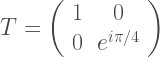
$T = \left( \begin{array}{cc} 1 & 0 \\ 0 & e^{i \pi / 4} \\ \end{array} \right)$
is transversal for the 15 qubit code, in the sense that
$T_{L}^\dagger = T^{\otimes 15}$ .
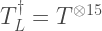However, there is a smaller colour code with only 8 physical qubits that is also interesting. Though the smaller code is a different flavour of interesting. The logical non-Clifford is a CCZ (control-control-Z), which is Clifford equivalent to a Toffoli.

Here, I want to describe this colour code and tell you about some intriguing connections to the topics of gate-synthesis and magic state distillation. Indeed, I discovered this curious code in the context of magic states, and it enables us to distill 8 noisy T-states into a less noisy CCZ magic state. This distillation protocol is essentially a different perspective on the results of Cody Jones and Bryan Eastin. Later, me and Mark Howard extended the construction to all gates in the third level of the Clifford hierarchy (see either the short paper or long paper). But I had an algebraic description of the code and I never noticed the code had a neat geometric representation as a colour code, which can be extended to higher distance colour codes (more on this later). Rather, at the FTQT Benasque meeting I was talking to Dan Browne and he described this colour code to me, and only then did I realise it was the same code I’d been working with. So I thank Dan for allowing me to steal his insight and turn it into a blog post.

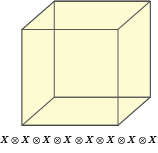
Onwards, to the description of the smallest interesting colour code. It is a [[8,3,2]] code. Translation: it uses 8 physical qubits to encode 3 logical qubits and has distance 2 (it can detect any one error, but not correct it). The geometric description of the rests upon a single cubic cell with 8 vertices, each corresponding to a qubit as follows:

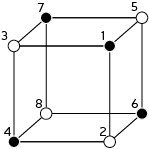
Note the numerical labels of qubits, which relate to the order of operators in tensor products used below. Also, I have two-coloured the vertices into black/white vertices, where black vertices are only adjacent to white vertices. The two-colorability of vertices is known to be directly related to the other colorability properties of colour codes (my preferred proof of this relation is Lemma 3 of [self-promoting link] ). Here, the relevance of two-colorability is that our transversal gate is achieved by applying $T$ to black vertices and $T^\dagger$ to white vertices, so that

$CCZ_{L1, L2, L3} = T \otimes T^\dagger \otimes T^\dagger \otimes T \otimes T^\dagger \otimes T \otimes T \otimes T^\dagger$

Notice that the logical CCZ involves the three logical qubits (labeled L1, L2, L3) of a single block of the 8 qubit code.

Now, lets define the code so we can verify these claims.

The Z stabilisers of the code corresponds to the face and cell operators of the cube. Only 3 face operators are needed to generate the stabiliser group. Other face operators emerge from group closure.

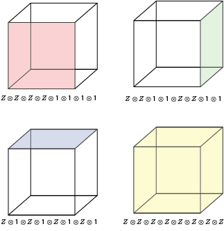
The sole X stabiliser of the code corresponds to the cell operators of the cube.

It is easy to check these all commute.

The logical X operators are membranes spanning the lattice. Yet, the lattice is a single unit cell and so a membrane is simply a face. The logical Z operators are strings spanning the lattice, and so are edges of this unit cell.

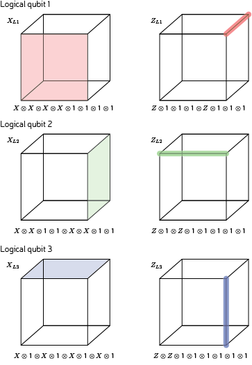
Again the relevant commutation and anti-commutation relations are easy to see in this geometric picture.

Having defined the code, there are many different ways to verify the transversality properties. Most mundanely, one can simply write out the computational basis states

$\vert (0,0,0)_L \rangle =\frac{1}{\sqrt{2}} (\vert 00000000 \rangle + \vert 11111111 \rangle )$
$\vert (1,0,0)_L \rangle =\frac{1}{\sqrt{2}} (\vert 11110000 \rangle + \vert 00001111 \rangle )$
… exercise to reader to fill in these states …
$\vert (1,1,1)_L \rangle =\frac{1}{\sqrt{2}} (\vert 10010110 \rangle + \vert 01101001 \rangle )$

and then check the transversality properties. For qubits in the $\vert 1 \rangle$ state, simply add a $\exp(i\pi/4)$ phase to black (even labelled) and a $\exp(-i\pi/4)$ phase for white (odd labelled) qubits. And out pops the CCZ gate.

The above calculation may not yield a great deal of intuition on the origin of CCZ transversality. A deeper understanding is reached by learning about a generalised notion of triorthogonal codes. Bravyi and Haah gave the original conception of triorthogonal codes to construct codes where the transversal gate is a logical $T$ . In our synthillation paper, we showed that this notion can be generalised to explain transversality of all gates in the Clifford hierarchy. While this proof encompasses CCZ gates, the proof’s generality may obscure the applicability to the above colour code. So let me paraphrase the argument for this special case (and slightly modify for a colored lattice). To get a CCZ logical we need:

All the X logical operators have support on an equal number of black and white vertices;
For any pair of X logical operators, the common support contains an equal number of black and white vertices;
For any trio of X logical operators, the common support contains an unequal number of black and white vertices, with the difference between an odd number;

One can easily check these conditions are satisfied on the cube unit cell. There are some additional demands on the X stabilisers, but these are very similar to the demands for transversality of a T-gate.

I also promised a connection to gate-synthesis, and this will explain why the code has 8 qubits! There are various papers (e.g. Amy and Mosca) that explain how to unitarily compose T gates with CNOT gates to implement any gate in the 3rd level of the Clifford hierarchy. For the CCZ gate, it is well known that 7 T-gates are optimal (at least without using any special tricks). Furthermore, this can be implemented in T-depth one (all 7 T gate are performed simultaneously) provided we use some ancillary qubits (first shown by Selinger). The CNOT gates preceding the T gates can be interpreted as an encoding unitary into some quantum code. However, the codes used by optimal gate-synthesis have no X-stabilisers, and so are distance one. The strategy me and Mark pursued was to take this trivial code and pad it out with extra qubits and extra stabilisers without harming its transversality properties. It transpires that for a circuit composed of solely CCZ gates (possibly very many CCZ gates), this padding is possible using only 1 additional qubit. Therefore, there is an error protected code using only one more qubit than optimal unitary gate-synthesis. 7+1=8, which explains the relation between the 8 qubit code and CCZ (which requires 7 T-gates). This post is skimming many details, but hopefully conveys a taste of the underlying mathematics. The full gory details appear in Example IV.1 of our paper.

Earlier in the post, I also alluded to higher distance colour codes. Here I was referring to unfolding the colour code by Kubica, Yoshida and Pastawski. This is a neat paper on the correspondence between colour codes and surface codes. However, buried within the paper is the observation that 3D colour codes (of large distance) can have CCZ transversality of the above nature. An important point is that the bulk lattice of a 3D colour code must be 4-valent, and this can only be violated at boundaries and defects. Therefore, these larger colour codes are not cubic lattices (which would be 6-valent in the bulk). However, the boundary conditions have some geometry and Kubica and company fix these boundaries to be cubic. Hence, we see that the smallest interesting colour code corresponds is an instance of this family of codes where the set of bulk qubits is empty. All qubits sit on the boundary.

This covers everything I wanted to say here. It has been a longer and more technical post than usual. But I think the connections between these different topics and papers is interesting and worth pointing out.

Reddit at FTQT

August 31, 2016September 24, 2016Leave a comment

Well the FTQT Benasque workshop has come and gone. It has a fantastic experience to spend two weeks with many smart people interested in quantum error-correction and fault-tolerance.

One of the unexpected, and unplanned from my perspective, things to happen was a Reddit Ask-Me-Anything. It was setup by James Wootton and several of us joined in, all sat in the same sofa area for a couple of hours. It was hilarious to hear someone gasp, “O no, someone has asked if quantum computing implies P=NP” quickly followed by “I’m on it!” from elsewhere in the room (I think Steve Flammia was the first on this one).

Below are a couple of photos of the AMA in progress. There are a few more pictures on the Benasque website. The lightening the main room wasn’t great and I only took my compact camera, so unfortunately a lot of pictures during talks went straight to trash.

Earl T. Campbell

Quantum wizardry, etcetera